Neural network simplified part 3 : learning
What differentiate Artificial Intelligence (AI) from other computer programs is their ability to learn; their behavior is not solely decided by programmers but also their own experience. This is why AI can outsmart us in many tasks. In this article, I will try to show you how neural networks (NNs) learn.
What it means to train a neural network (NN)
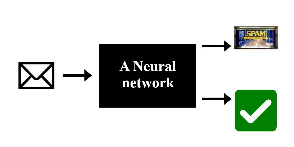
Let’s remind ourselves of the first article where I presented a simple NN to classify mails as spam or not spam. These kinds of NNs take in some numbers and output others. Here, the input represents a mail in some way (style, spelling, grammar, …) and the output represents how much the network thinks this mail is spam.
In the first article, I also explained how NNs make decisions. To summarize, neurons are linked and these linked have an associated weight. The weight of each link decides how strongly the information flows from one neuron to the next. Hence, the weights completely define how the network behaves.
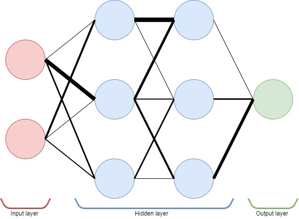
To train a NN is to find an arrangement of weight, where some neurons are more strongly linked than others, such that the network makes good decisions. Note that many different arrangements of weight can lead to the same performance due to the internal symmetry of NN.
Supervised learning
Supervised learning is one way that we can train NNs. It means we use labelled data to train our network. In this case, imagine we have 10000 mails manually labelled by someone as spam or not spam. We will present this data to the network, so it can learn to differentiate the two kinds of mail.
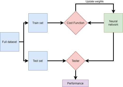
In practice, we usually cut the data in multiple sets. A training set is used to train the network and a test set is used to test its performance. Indeed, since the network is trained on the training set, it knows the data and will perform better on it. Thus, keeping a separate test set ensures the network is tested on data it has never seen. This gives a better measure of the performance of the network.
The influence of weights on the error
What we want is to reduce the overall error the network makes. Here, this means reducing the misclassification of mails. Imagine a machine that takes in the NN current weights and outputs the error for a given training set; this machine is called the cost function. Hence, what we want is to minimize the cost function by choosing a better set of weights.
The weights are a set of numbers. Let’s first imagine there is only one. At any time we can increase or decrease this weight and this will affect the error on the training set. Hence, there exists for this weight at least one value that leads to the lowest error (marked as a green X on the graph below). In practice however, we do not have one weight but often millions but the idea is the same : there is an error curve and a point at which it is lowest and the goal is to find it.
While in theory we can draw the cost function, in reality we can only know the error for tested weight configurations. This means we do not know what the cost function looks like. Hence, we do not know right away what the best weight configuration is. Thus, we need training protocols to look for weight configuration that leads to good performance.
[the_ad id=”1647″]
Training protocols
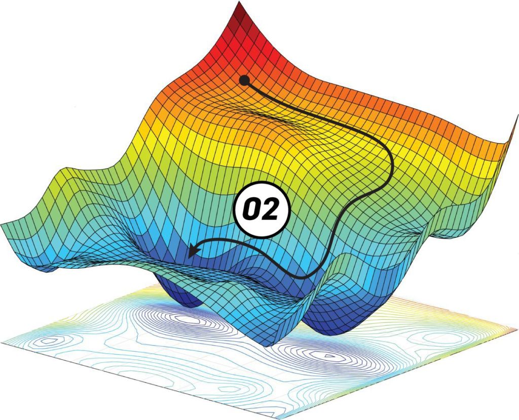
A naive approach is to test many weight configurations randomly chosen and pick the best but this is painfully slow and inefficient. A better approach yet is gradient descent. I won’t get into the details but here the magic of mathematics gives us a nice tool : gradient. Gradients can give us the direction of local descent for a given function. Thus, there is no need to look in a few directions. We now have a nice way to reduce the error by following this gradient, it’s fast to compute and much more efficient. If we follow the gradient, we are guaranteed to arrive at a local minima of the cost function.
One big problem with descent methods is that we risk getting stuck in a local minimum. This is because the cost function has a complex shape and there are many valleys and dune. We want to get down the lowest valley, but we can only see locally. Hence, if we are in a local minimum, we are stuck there because the only way out is to climb up. We can’t climb up because we want to go down and remember in practice you do not know what the complete error curve looks like.
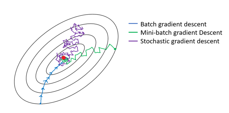
Stochastic gradient descent was invented to alleviate this issue. Again, let’s not get into the details but imagine that instead of the error curve being static, we vibrate it with some intensity. This means sometimes, when stuck in a small valley, a wave will come and the valley becomes a hill you can fall down from. The error curve vibrates just a bit and always keeps a somewhat similar shape such that large valleys do not disappear and only small ones are affected. This solution is much more efficient because it allows us to avoid getting stuck in some local minima. It is the basis of most learning protocols currently in use. Yet, it can take weeks to train some networks.
Conclusion
Neural networks need to learn. This means finding a set of weights to minimize the cost function. With the help of labelled data, we can use training protocols such as stochastic gradient descent to find a good set of weights. This is similar to exploring a surface to find the lowest valley.
Oh, I see you’ve read till the end. Thank you for your support; I hope this series is interesting. If you want to tinker with NN, I suggest you go to the playground where you can play around with a simple NN and a few datasets. Have fun adding layers, neurons, testing stuff, etc. It’s great fun. I highly recommend it.

Is your company looking to integrate AI solutions, analyze data, or strengthen its back-end development? Contact me!
Mail : pro.judicael.poumay@gmail.com
Linkedin : Judicaël Poumay
Portfolio : www.portfolio.thethoughtprocess.xyz
Spinoff project : www.aiashi.be
- Why non linearity matter in Artificial Neural Networks - 18 June 2024
- Is this GPT? Why Detecting AI-Generated Text is a Challenge - 7 May 2024
- The Transformer Revolution: How AI was democratized - 21 February 2024